Conditional Probabilities and Bayes

Conditional Probabilities

• Let’s say we are looking at the likelihood that someone knows R in the Bienen School of Music.

• We know there are about 700 people in Bienen School of Music, and it’s safe to say that maybe 10 know R.

Conditional Probabilities

• \(P(knowingR) = \frac{8}{700}\)
  • The probability of knowing R in Bienen is 8 out of 700.
• \(P(knowingR|thisClass) = \frac{13}{700}\)
  • The probability of knowing R in a quarter in which this class is offered, is 13 out of 700.
• \(\frac{P(knowingR|thisClass)}{P(knowingR)} = 1.625\)
  • What does this tell us? In a quarter that this class is being offered, you’re 62.5% more likely to find someone who knows R.

Conditional Probabilities

• On the individual level, it’s still quite rare to know R, but at the population level, it goes up quite a bit.

“Conditional probabilities are an essential part of statistics because they allow us to demonstrate how information changes our beliefs.” (Will Kurt)

Dependence and the Revised Rules of Probability (taken from Kurt)

• \(P(colorBlind) = .0425\)
• \(P(colorBlind|female) = .005\)
• \(P(colorBlind|male) = .08\)
• If we pick someone at random, what are the odds that they are male and color blind?

Dependence and the Revised Rules of Probability (taken from Kurt)

• This would be the basic population equation:
  • \(P(male, colorBlind) = P(male) * P(colorBlind)\) =
    • .5 * .0425 = .02125
  • But this doesn’t really answer the full question.
• These are dependent probabilities.
  • The true probability of finding a male who is color blind is the probability of picking a male multiplied by the probability that he is color blind.
  • \(P(male, colorBlind) = P(male) * P(colorBlind | male)\)
  • .5 * .08 = .04
  • \(P(A,B) = P(A) * P(B|A)\)

Dependence and the Revised Rules of Probability (taken from Kurt)

How can we determine the \(P(male|colorBlind)\)?

• \(P(male|colorBlind) = \frac{P(male) * P(colorBlind|male)}{P(colorBlind)}\)
• = \(\frac{.5 * .08}{.0425}\)
• = .941

Bayes’ Theorem

• \(P(A|B) = \frac{P(A) * P(B|A)}{P(B)}\)
• Allows us to look at the likelihood of what we’ve seen given what we believe.
• \(P(observed|belief)\) as well as \(P(belief|observed)\)

Bayes’ Theorem

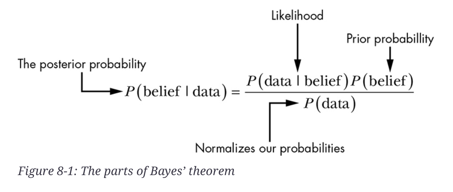
Kurt figure 8.1

We’ve been robbed (taken from Kurt again)

• P(robbed | broken window, open front door, missing laptop)

• What are the odds that, if you were robbed, you’d come home and find this evidence? 3 out of 10?

• \(P(robbed) = \frac{1}{1000}\)

• \(P(robbed) * P(brokenWindow, openDoor, missingLaptop|robbed)\)

  • = \(\frac{\frac{1}{1000} * \frac{3}{10}}{P(D)}\)

We’ve been robbed (taken from Kurt again)

• The problem is, we don’t really know P(D)
• But perhaps we can compare hypotheses?

We’ve been robbed (taken from Kurt again)

1. Kid hit a baseball through the front window
2. I accidentally left the door unlocked.
3. Forgot that I brought the laptop to work and it’s still there.

We’ve been robbed (taken from Kurt again)

• P(kid) = 1/2000
• P(door) = 1/30
• P(laptop) = 1/365
• \(P(H_2) = \frac{1}{2000} * \frac{1}{30} * \frac{1}{365}\)
  • = 1 out of 21,9000,000.

Comparing Hypotheses

• \(\frac{P(H_1) x P(D | H_1)}{P(H_2) x P(D | H_2)}\)

• \(\frac{\frac{3}{1000}}{\frac{1}{21,900,000}}\)

• = 6,570

• \(H_1\) explains what we observed 6,750 times better than \(H_2\).

• Our original hypothesis explains the data much, much better than the second hypothesis.

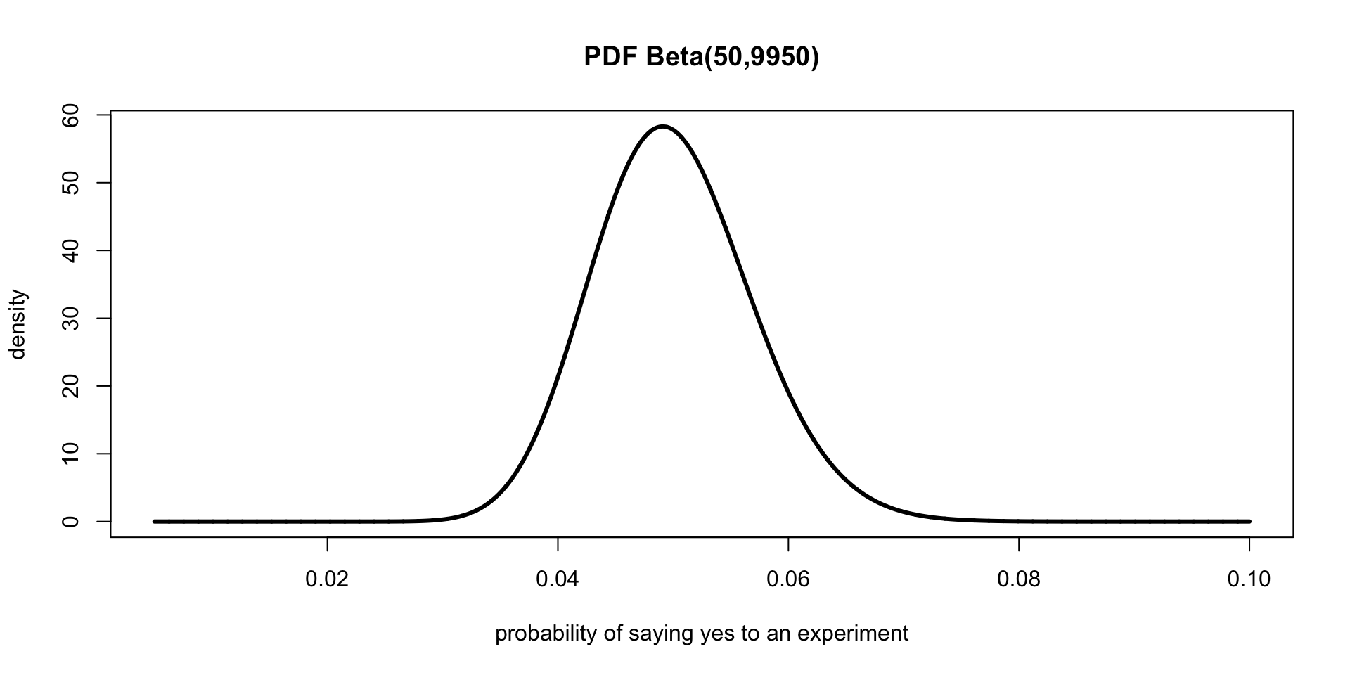
The beta distribution

• Let’s say that I need to get students at NU to do an experiment.
• I ask 10,000 people.
• I get 50 people to say yes.

The beta distribution

Schemata or Not

	Found Schema	Didn’t Find Schema	Accuracy Rate
Orchestral	36	114	.24
Piano	50	100	.33

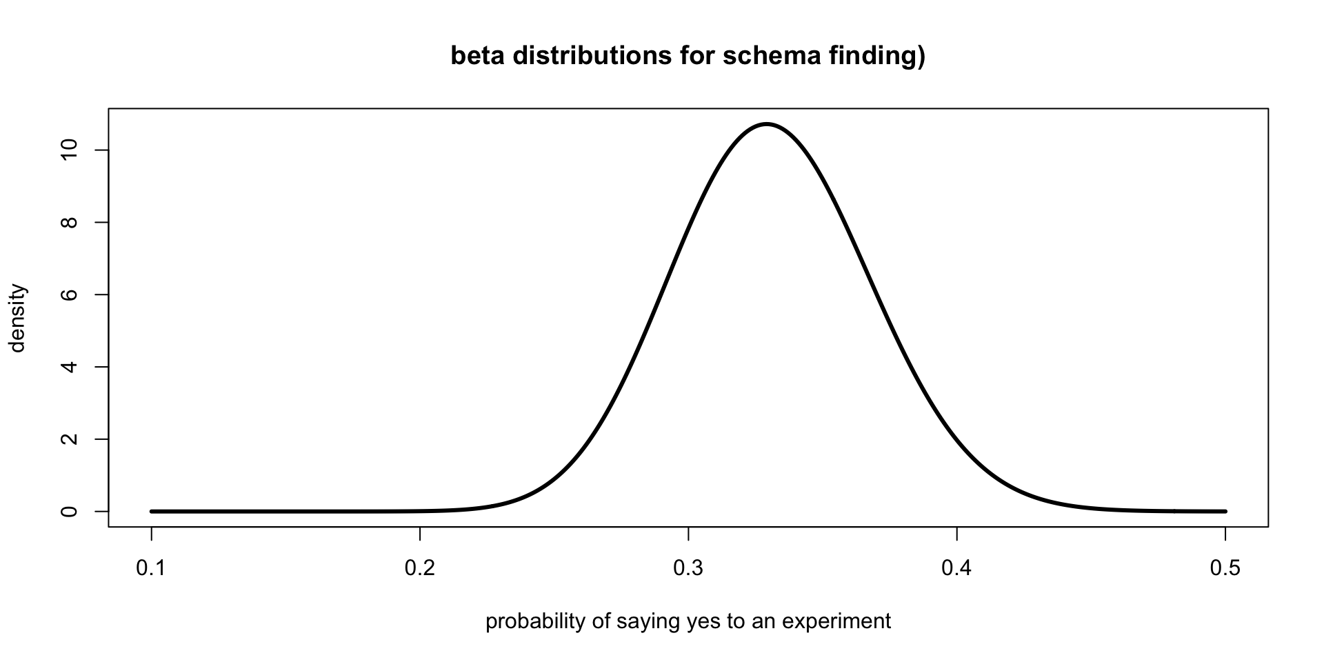
Schemata or Not

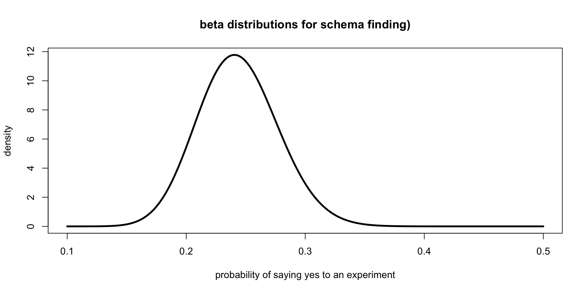
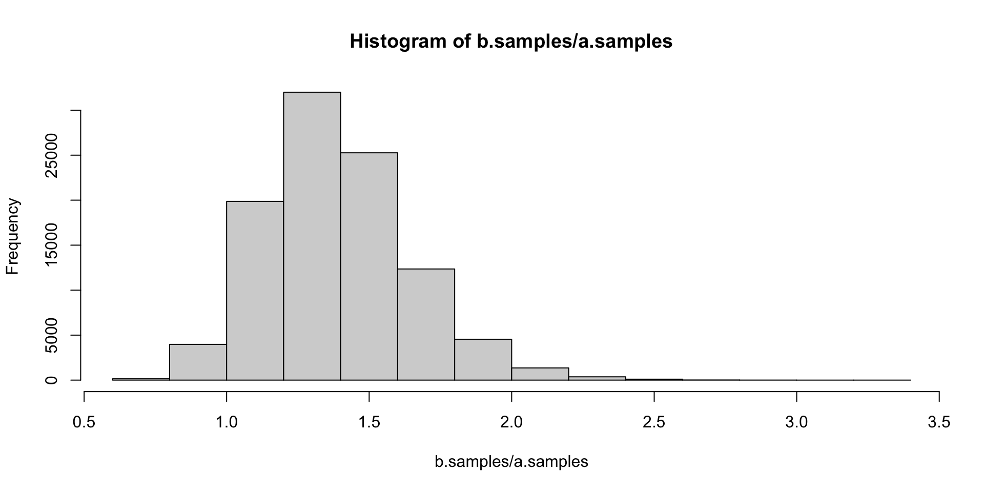
another distribution

Monte Carlo Simulation

[1] 0.95875